# read the JSON file, convert to data frame, and unnest some columns
read_json(list.files()[grep(".jscor", list.files())], simplifyVector = TRUE) |>
  as.data.frame() |>
  unnest(cols = c(games_attributes.sixths_attributes,
                  games_attributes.final_attributes),
         names_repair = "universal") |>
  # keep only regular difficulty games
  filter(!games_attributes.play_type %in% c("toc", "masters")) |>
  # keep only the columns we need, add a round indicator, pivot to one row per
  # clue instead of per category, and calculate each clue's contribution to the
  # Coryat score
  select(2, 10:14) |>
  mutate(round = rep(c(rep(1, 6), rep(2, 6)), n()/12)) |>
  pivot_longer(cols = 2:6, names_to = "clue", names_prefix = "result") |>
  rename(result = value) |>
  mutate(result = recode(result, `1` = -1, `3` = 1, `7` = 1, .default = 0),
         score = round * as.numeric(clue) * 200 * result) |>
  # group by game, add up the total score, sort by game order, and throw away
  # the time stamps
  group_by(games_attributes.date_played) |>
  summarize(sum(score)) |>
  arrange(1) |>
  mutate(game = row_number()) |>
  select(-1) |>
  rename(score = `sum(score)`) ->
  # store the results
coryat_scoresCoryat Scores
The joy of Jeopardy! judgement.
Introduction
Coryat Scores
The Coryat score is a way of measuring one’s performance when playing along with Jeopardy! at home. It is named after musician, philosopher of physics, and two-day Jeopardy! champion Karl Coryat.
A player’s Coryat score is the total value of clues answered correctly, minus that of those answered incorrectly, counting correctly-answered Daily Doubles according to their board position and ignoring Final Jeopardy! and any incorrectly-answered Daily Doubles.
Thus the Coryat score is a measure of one’s knowledge of the trivia material used on the show, ignoring other strategic elements like wagering.
J! Scorer
J! Scorer is a convenient way to record games and determine one’s Coryat score. The site was created by two-time TV game show contestant Steve McClellan and has a public GitHub repository.
J! Scorer users can download a JSON file of their games.
Data
It took a little effort to reverse-engineer the format of the files produced by J! Scorer. (I did this before finding the above-mentioned GitHub repo.) I used jsonlite::read_json plus a little trial and error. Then it’s just a matter of straightforward data transformations using dplyr.
Table
coryat_scores |>
  kable(caption = "My Jeopardy! Coryat Scores") |>
scroll_box(height = "5in")| score | game |
|---|---|
| 17800 | 1 |
| 10200 | 2 |
| 16000 | 3 |
| 12400 | 4 |
| 16400 | 5 |
| 16800 | 6 |
| 18200 | 7 |
| 16000 | 8 |
| 16000 | 9 |
| 18400 | 10 |
| 18600 | 11 |
| 22600 | 12 |
| 25000 | 13 |
| 17600 | 14 |
| 19600 | 15 |
| 24000 | 16 |
| 19600 | 17 |
| 18600 | 18 |
| 20200 | 19 |
| 17800 | 20 |
| 26800 | 21 |
| 21000 | 22 |
| 20800 | 23 |
| 19600 | 24 |
| 17800 | 25 |
| 18200 | 26 |
| 16600 | 27 |
| 25400 | 28 |
| 4000 | 29 |
| 27800 | 30 |
| 18600 | 31 |
| 27000 | 32 |
| 24200 | 33 |
| 21600 | 34 |
| 22600 | 35 |
| 21400 | 36 |
| 18800 | 37 |
| 11800 | 38 |
| 23200 | 39 |
| 28000 | 40 |
| 24400 | 41 |
| 14800 | 42 |
| 17000 | 43 |
| 16200 | 44 |
| 27800 | 45 |
| 18000 | 46 |
| 18200 | 47 |
| 28600 | 48 |
| 22600 | 49 |
| 13600 | 50 |
| 18000 | 51 |
| 16200 | 52 |
| 18400 | 53 |
| 17200 | 54 |
| 24200 | 55 |
| 19400 | 56 |
| 20400 | 57 |
| 21000 | 58 |
| 16800 | 59 |
| 19800 | 60 |
| 24800 | 61 |
| 19600 | 62 |
| 20400 | 63 |
| 24400 | 64 |
| 18600 | 65 |
| 17200 | 66 |
| 23400 | 67 |
| 26600 | 68 |
| 24800 | 69 |
| 21600 | 70 |
| 24600 | 71 |
| 21600 | 72 |
| 17600 | 73 |
| 12000 | 74 |
| 21600 | 75 |
| 17800 | 76 |
| 23600 | 77 |
| 21800 | 78 |
| 22400 | 79 |
| 18800 | 80 |
| 28400 | 81 |
| 16800 | 82 |
| 21400 | 83 |
| 5600 | 84 |
| 15000 | 85 |
| 19400 | 86 |
| 14200 | 87 |
| 16400 | 88 |
| 23200 | 89 |
| 20400 | 90 |
| 22600 | 91 |
| 18200 | 92 |
| 14000 | 93 |
| 17000 | 94 |
| 19000 | 95 |
| 18400 | 96 |
| 18400 | 97 |
| 26200 | 98 |
| 26400 | 99 |
| 22800 | 100 |
| 33200 | 101 |
| 19800 | 102 |
| 26400 | 103 |
| 18600 | 104 |
| 13600 | 105 |
| 22200 | 106 |
| 24800 | 107 |
| 27400 | 108 |
| 13400 | 109 |
| 14000 | 110 |
| 13600 | 111 |
| 15200 | 112 |
| 12000 | 113 |
| 20800 | 114 |
| 26200 | 115 |
| 16800 | 116 |
| 20400 | 117 |
| 28800 | 118 |
| 32400 | 119 |
| 10400 | 120 |
| 20000 | 121 |
| 12400 | 122 |
| 11400 | 123 |
| 20600 | 124 |
| 19800 | 125 |
| 18200 | 126 |
| 20200 | 127 |
| 20000 | 128 |
| 15800 | 129 |
| 16400 | 130 |
| 17000 | 131 |
| 22400 | 132 |
| 15600 | 133 |
| 20200 | 134 |
| 20600 | 135 |
| 18600 | 136 |
| 19400 | 137 |
| 22800 | 138 |
| 13400 | 139 |
| 18800 | 140 |
| 15200 | 141 |
| 20000 | 142 |
| 14000 | 143 |
| 25200 | 144 |
| 25800 | 145 |
| 20000 | 146 |
| 28600 | 147 |
| 16200 | 148 |
| 16400 | 149 |
| 18000 | 150 |
| 20200 | 151 |
| 18600 | 152 |
| 19800 | 153 |
| 13000 | 154 |
| 10200 | 155 |
| 15600 | 156 |
| 14400 | 157 |
| 25200 | 158 |
| 26800 | 159 |
| 14800 | 160 |
| 21400 | 161 |
| 16800 | 162 |
| 19200 | 163 |
| 17600 | 164 |
| 20800 | 165 |
| 25000 | 166 |
| 27400 | 167 |
| 20800 | 168 |
| 20000 | 169 |
| 26800 | 170 |
| 22800 | 171 |
| 33800 | 172 |
| 16600 | 173 |
| 20800 | 174 |
| 20800 | 175 |
| 27800 | 176 |
| 19200 | 177 |
| 16200 | 178 |
Average Score
An average score of around $25,000 is considered appropriate for prospective contestants.
# calculate my mean score
coryat_scores |> pull(score) |> mean() |> round()
[1] 19787Clearly, I have some studying to do before I consider trying to compete on the show.
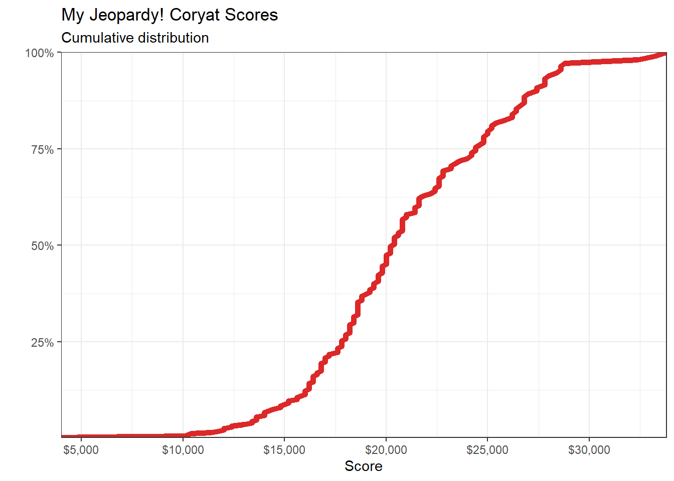
Visualization
We can create a histogram showing the distribution of my scores and a line chart showing the evolution of my scores over time using ggplot2.
Code
# main plot
(coryat_scores |>
  ggplot() +
  # aesthetic mapping
  aes(x = game, y = score) +
  # visual elements representing the data
  geom_line(colour = "#b4b4b4") +
  geom_smooth(se = FALSE, colour = "black") +
  geom_hline(yintercept = 25000, linetype = "dashed") +
  geom_point(colour = "#dc2828") +
  # scales
  scale_y_continuous(labels = scales::label_dollar(),
                     n.breaks = 6,
                     limits = c(0, 30000)) +
  scale_x_continuous(expand = c(0, 0), breaks = NULL) +
  # labels
  labs(title = "My Jeopardy! Coryat Scores",
       subtitle = "Trend and distribution",
       x = "",
       y = "Score",
       caption = "Dashed black line indicates target average of $25,000.") +
  # theming
  theme_bw()) |>
  # add the marginal histogram
  ggMarginal(type = "histogram", margins = "y", fill = "#b4b4b4")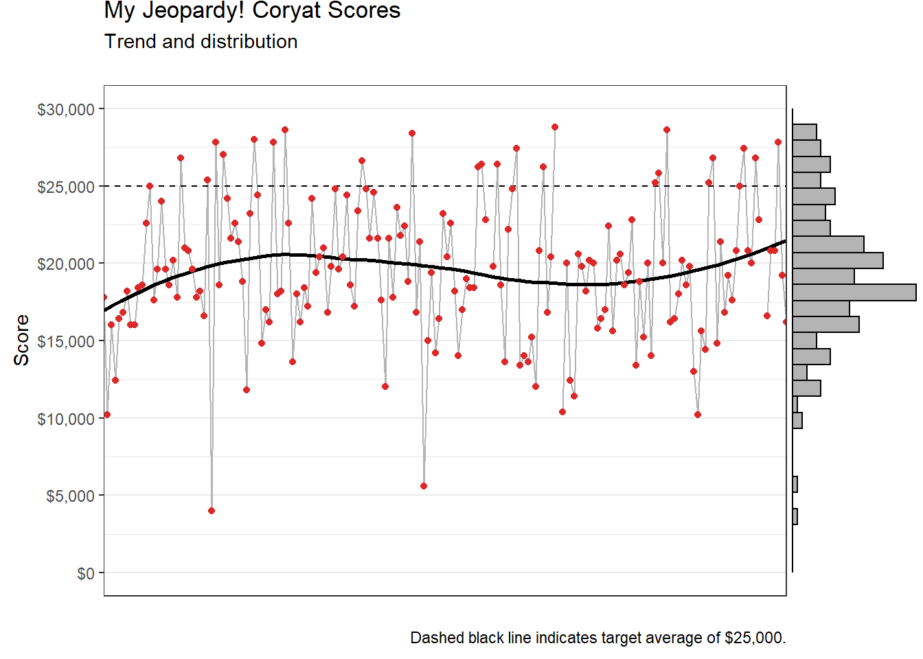
Code
coryat_scores |>
  arrange(score) |>
  ggplot(aes(x = score, y = cumsum(score)/sum(score))) +
  geom_line(size = 2, colour = "#dc2828") +
  scale_x_continuous(labels = scales::label_dollar(),
                     n.breaks = 6,
                     expand = c(0, 0)) +
  scale_y_continuous(labels = scales::label_percent(), expand = c(0, 0)) +
  labs(title = "My Jeopardy! Coryat Scores",
       subtitle = "Cumulative distribution",
       x = "Score",
       y = "") +
  theme_bw()